
Portions of the text below have been excerpted from the following NALMS publications:
Carlson, R.E. and J. Simpson. 1996. A Coordinator’s Guide to Volunteer Lake Monitoring Methods. North American Lake Management Society. 96 pp.
Temperature
There are a number of basic reasons for measuring temperature in lakes. Thermal structure is a dominant factor affecting many lake processes of interest to limnologists.
Temperature Classification of Lakes
At the very least, temperature is the basis of a thermal classification of a lake. A thermal classification can help the coordinator separate lakes with similar thermal structures, and, in doing so, perhaps into groups of similar function as well.
The thermal classification scheme of Hutchinson and Löffler (1956) and Hutchinson (1957) is commonly used. This scheme, summarized in Table 1, first divides lakes into classes based on those that undergo complete circulation and those that do not.
- Amictic lakes are permanently ice-covered and do not circulate.
- Holomictic lakes circulate throughout the entire water column at some time during the calendar year.
- Dimictic lakes have a summer stratification and also a winter stratification under the ice, circulating only during the spring and fall.
- Polymictic lakes stratify irregularly throughout the year, being either very large lakes in colder climates that have minimal ice cover during the winter (cold polymictic) or lakes in tropical or sub-tropical regions that stratify irregularly throughout the year (warm polymictic).
- Meromictic lakes do not undergo complete circulation: often the lower portion has a chemically-induced density difference with the upper waters and is perpetually separated from the overlying water (Hutchinson 1957; Wetzel 1975).
Holomictic lakes were subdivided into monomictic, dimictic, and polymictic lakes. Monomictic lakes only stratify once during the year. Warm monomictic lakes circulate only during the winter, having a thermal stratification during the summer, while cold monomictic lakes remain near 4 °C throughout the year but circulate only during the summer.
Unfortunately, this classification scheme does not adequately address the problem of the temperate shallow lake (Wetzel 1975), although these lakes are common in North America. They have ice cover during the winter and therefore have a period of thermal stratification, which should classify them as monomictic. However, during the ice-free season, they may not stratify at all or may have periods of stratification interspersed with periods of free circulation. Wetzel (2001) recommends the use of a modification of the scheme by Lewis (1983), which is presented in Table 1. In this classification, these shallow lakes would be classified as polymictic, but as Wetzel points out, even polymixis is based on frequency of thermal stratification, and lakes that do not thermally stratify really do not fit well within the classification.
This classification does more than provide another label for a lake; it also provides insights into how the lake might function. The typical north-temperate first-class and second-class dimictic lake has a distinct thermocline during the summer. During that stratified period, oxygen may or may not decline to zero in the hypolimnion. The effects of this anoxia can be profound, depending on the thermal stability of the lake. Stability of a lake is defined as the amount of work needed to mix the entire body of water to a uniform temperature without addition or subtraction of heat (Schmidt 1915, 1928; Hutchinson 1957). This stability can be estimated or indexed by several equations, all of which require detailed thermal information that could be obtained by volunteers. In the various forms of polymictic lakes, the degree of thermal stability is minimal or absent. In this case, the sediments are continually or intermittently exposed to the epilimnetic waters. Oxygen concentrations near the sediments may fluctuate daily, depending on the degree of daily mixing of the epilimnion.
It is also possible that, during the brief periods of thermal stability in polymictic lakes, that oxygen will disappear near the sediments. During these periods of anoxia, phosphorus may be released from the sediments and build up in the lower strata. When the stratification disappears, this nutrient-laden water will be mixed into the upper water where it may stimulate algal growth. These lakes may be characterized by periodic peaks or pulses in phosphorus and algae throughout the ice-free season.
| Table 1. The thermal classification scheme of Hutchinson and Löffler (1956) and Hutchinson (1957) as modified by Lewis (1983). | |
| Amictic | Sealed permanently by ice. |
| Monomictic | Lakes that only circulate once during the year. |
| Warm monomictic | Lakes that circulate freely during the winter, having a stable thermal stratification during the summer. |
| Cold monomictic | Lakes that remain near 4 °C throughout the year but circulate only during the summer. |
| Dimictic | Lakes that are thermally stratified during the ice-free season, circulating freely in the spring and fall. |
| Polymictic | Lakes that stratify irregularly throughout the year |
| Continuous Cold Polymictic | Lakes have a winter ice cover, and during the ice-free season, circulation is continuous or only interrupted by brief diurnal periods of stratification. |
| Discontinuous Cold Polymictic | Lakes have a winter ice cover, and during the ice-free season, is thermally stratified except for brief periods of circulation. |
| Discontinuous Warm Polymictic | Lakes that have no seasonal ice cover and thermally stratify for day or weeks at a time, but mixing more than once a year. |
| Continuous Warm Polymictic | Lakes with no ice cover that mix continuously throughout the year except for brief (hours) periods of stratification. |
| Meromictic | Lakes that do not undergo complete circulation, usually because of a stable thermal or chemical layer near the bottom. |
Identification of Seiches
Frequent temperature measurements can also detect the presence of internal seiches in lakes. A steady wind blowing down a lake, a change in air pressure, or a localized storm on a big lake can set the water to rocking with a characteristic period. This rocking of the lake water back and forth is called a seiche. Surface seiches can be detected by changes in water height, but another type of seiche is set up, not at the water surface, but at the thermocline. These internal seiches can rock back and forth for many days. As the water moves back and forth, some of the deeper water, which can be rich in nutrients, is mixed into the upper water. Thus the seiche helps fertilize the upper waters and provide the nutrients necessary for algal growth. The effect is accentuated in long, narrow lakes and reservoirs. Either a height recorder or a large number of lake height observations can be used to measure the range and period of a seiche, but frequent temperature measurements at one end of a narrow lake may reveal an internal seiche.
Quantification of the Thermocline
Probably most volunteer programs simply plot temperature over time or depth without considering that there is a wealth of other valuable information available that is being ignored. It is possible to easily quantify the depth of the thermocline and even the depth of the top and bottom of the metalimnion. This information can be used to alter sampling depths if sampling depends on thermocline depth or depth of the epilimnion. The information can also produce an easily interpretable graph of how and when the thermocline sets up and declines.
If you calculate the rate of change in temperature, the thermocline is defined as the point of maximum rate of change (Fig. 1a and 1b). This is easily calculated on a spreadsheet by taking the difference in temperature at two consecutive depths. This difference is divided by the difference in depth. The resulting value is the rate of change in temperature. The equation is:
ΔT/Δz = (Tn – Tm) / (n – m)
where Tn and Tm are the temperatures at the top (n) and bottom (m) of a given slice of the depth of the water. The results are plotted in Fig. 1b. The maximum change in temperature, represented by the peak at, in this case, 5 meters, is the defined thermocline.
The top and bottom of the metalimnion are defined as the minimum and maximum of the second derivative of the change in temperature These values are easily calculated as the rate of change of the rate of temperature change calculated above; subtract the rate of change in temperature at two consecutive depths and divide this difference is divided by the difference in depth. The results, shown in Fig.1c, show the top of the thermocline to be at 4 m and the bottom at 6 m.
 |
 |
 |
|
| Figure 1. Going beyond a simple plotting of temperature versus depth (1a). Taking the first and second derivative of temperature allows you to estimate the depth of the thermocline (1b) and the upper and lower bounds of the metalimnion (1c). | |
With these values of the thermocline depth and the upper and lower bounds of the metalimnion, you can easily plot the seasonal change in the depth of the thermocline and the width of the metalimnion.
Measuring Temperature
A number of methods exist for measuring temperature, with costs ranging from a few dollars to several hundreds of dollars. The simplest method requires only an accurate thermometer, preferably one with a metal or plastic shield that minimizes the possibility of breakage. When a thermometer is used, water has to be brought up from the desired depths, the thermometer inserted, and, after a period of equilibration, the temperature read. Care must be taken so that the temperature does not change during the time from sampling to the time the temperature is read. This might be accomplished by rapidly bringing the water up from the depth, using an insulated or thick plastic sampling container, and minimizing the time of exposure of the enclosed sampler to the ambient air temperature.
An alternative method is to have the thermometer permanently embedded in the sampler, either at the top or fixed to the inside of a clear sampler. In this case, all the volunteer has to do is take the sample, bring it to the surface, and read the thermometer. Again, the coordinator must be certain that the apparatus is constructed in such a manner that the temperature of the sample does not change significantly during its assent.
Temperature information can also be gained by drop a weighted maximum-minimum thermometer to the desired depth (Lind 1985). The max-min thermometer is constructed in such a way that the maximum temperature (air or surface water) and the minimum temperature (the temperature at depth) will be recorded. If the lake is “normal,” and temperatures decrease continuously with depth, a series of measurements of the minimum temperatures should accurately reflect the temperature profile of the lake. However, difficulties arise if there is an inverted temperature structure and colder temperatures overly warmer temperatures, as does happen near the bottom during ice-cover.
The most convenient method for measuring temperature is using an electric thermistor thermometer. This device works on the principle that temperature changes the resistance of a wire to an electric current. In these instruments, the only sensitive portion of the wire is the tip, or probe. The wire is simply lowered to the desired depth, the probe allowed to equilibrate, and the temperature measurement taken. Although the instrument is convenient, especially when coupled with an oxygen probe (see next section), it is important to calibrate the instrument against an accurate laboratory thermometer over the entire temperate range encountered in the lake.
It is also important that batteries of the thermistor not be allowed to decline in output. If the instruments are calibrated and fresh batteries installed in the spring, it may be that their accuracy will remain high throughout the summer season, but the coordinator should be sure that this is the case. Thermistor instruments range in costs from $40.50 for fishermen’s models up to several hundred dollars for scientific instruments. It might be expected that accuracy varies proportional to cost, but this needs to be examined.
Oxygen
Hypolimnetic oxygen concentration has long been considered to be an important indicator of eutrophication. With increased nutrient concentrations in the epilimnion and the subsequent increase in plant biomass, the amount of organic material injected into the hypolimnion increases as well. In a stratified lake, these increased organic loads increase the decomposition rates and, subsequently, the rate of oxygen depletion. The depletion of oxygen from the hypolimnion can cause a number of significant changes in the chemistry and biology of a lake. The loss of oxygen will be accompanied by lower oxidation-reduction potentials in the bottom waters, and the appearance of a number of soluble reduced compounds, including iron and manganese.
If phosphorus, previously bound to iron hydroxy complexes, is released, it may find its way through the thermocline, providing a potentially significant internal source of phosphorus to the epilimnetic plants. With an internal source of phosphorus provided for the plants, it is possible that a positive feedback system can be generated, with the hypolimnion providing the phosphorus, and the plants providing the organic matter that contributes to the oxygen depletion.
Decreased oxygen also causes the loss of hypolimnetic and benthic species of plants and animals. Perhaps the most obvious changes would be the loss of salmonid fishes such as lake trout, but a number of other hypolimnetic species will be either lost or forced into the epilimnion. For example, the decline of the copepod, Limnocalanus macrurus, in Lake Michigan was thought to be the result of decreased oxygen levels forcing the species into the metalimnion, where they were subjected to intense predation by alewives (Gannon and Beeton 1971). In fact, one of the earliest trophic classifications was based on the shift from the chironomid genus, Tanytarsus to the genus Chironomus as a lake lost its hypolimnetic oxygen (Rodhe 1975).
Trophic classification of lakes has often been made solely on the presence or absence of oxygen in the hypolimnion, but this method is subject to error because the oxygen does not deplete immediately upon thermal stratification; the depletion rates depend, not only on the organic load, but the oxygen concentration during turnover, the temperature of the hypolimnion, and the morphometry and size of the hypolimnion relative to the size of the epilimnion (Hutchinson 1957). The presence or absence of oxygen will also depend on when the hypolimnion is sampled relative to the time of stratification.
The rate of oxygen depletion is a more useful measure than presence/absence information, but does require samples to be taken periodically throughout the stratified period. The simplest measure of oxygen depletion rate is the relative oxygen deficit (Hutchinson 1957). This is obtained by subtracting the actual hypolimnetic oxygen concentration on a given day from the oxygen concentration during spring turnover. Hypolimnetic oxygen concentration is obtained weighting concentrations by water volume at a series of depths in the hypolimnion. Either a plot of the relative deficit against time or a straight line calculation between oxygen concentration at turnover and a date later in the summer will provide an estimate of the rate of oxygen depletion.
Another measure of oxygen depletion is the hypolimnetic areal deficit (Hutchinson 1957). This index is the mean relative deficit below 1 square centimeter of hypolimnetic surface. The calculation of the deficit relative to hypolimnetic area compensates for lakes with different sized hypolimnia. In doing so, it allows for more accurate comparisons of deficits between lakes. Its calculation is relatively simple. The areal deficit is calculated as above, but the rate of depletion is then divided by the hypolimnetic area (cm2). An example of its calculation is given in Wetzel (1975). However, even the hypolimnetic areal deficit does not compensate for differences in organic loading from humic substances or from temperature, and therefore is still a relatively inaccurate index of trophic state, especially in lake-to-lake comparisons.
Oxygen deficits are often used as indicators of trophic state, but this seems to be a waste of good information. Oxygen deficits make a poor indicator of trophic state because deficits are affected by many non-trophic state related factors such as organic loading, temperature, and morphometry. Lakes with high organic loadings of detritus or humic materials, second class dimictic lakes, lakes at lower latitudes, and those with a small hypolimnion relative to the epilimnion would be classified as eutrophic based on their oxygen deficits even though the amount of nutrient loading, nutrient concentration, or amount of plant material were identical. Trophic state can be determined much more easily and accurately by a number of other variables.
The rate at which oxygen disappears from the hypolimnion is an important piece of information both to understand the dynamics of a lake and for its management, especially if that rate is quantified and tracked from year to year. Oxygen deficits are most often used to compare different lakes, but differences in morphometry, geographic location, and trophic state can make the comparisons less useful. However, if yearly measurements are made on the same lake, then morphometry and location become constants in the relationship.
One would expect that, as a lake eutrophies, the rate of oxygen consumption in the hypolimnion would increase. This would happen for two reasons. First, because more algae and macrophytes would be produced in the epilimnion, it would be expected that more organic material would settle into the hypolimnion and decompose there. Second, some of the material would not be completely decomposed and would settle onto the sediments. In the following years, the decomposition of the organic sediments would also place a demand on the oxygen supply of the hypolimnion. The initial disappearance of oxygen in the hypolimnion can occur prior to any noticeable change in the productivity of algae in the epilimnion because of the amplification of organic epilimnetic inputs by the sediments (Gliwicz and Kowalczewski 1981). This makes the oxygen content of the hypolimnion and the rate of disappearance to be a potential “early warning system” of changes in trophic state.
Measuring Oxygen
As with temperature, several methods exist for measuring oxygen, with widely-ranging costs. Considerations include convenience, time, accuracy, and safety.
The least expensive method involves the chemical determination of oxygen in a water sample. The usual technique used is called the modified Winkler technique. Water has to be brought up from the desired depth in a water sampler such as a Kemmerer or Van Dorn bottle, a known volume poured into a glass container, reagents added, and, finally, the sample titrated. Although limnologists usually do this procedure in the laboratory, several companies make relatively simple field test kits that would allow a volunteer to perform the test. What is sacrificed with these test kits may be accuracy, because, while the test is similar to that used in most limnological laboratories, the titration burette used in the laboratory may be replaced by an eye dropper or a syringe. While accuracy may be sacrificed, the loss may not be that important to a volunteer program, where the presence or absence of oxygen, not its concentration, accurate to the first decimal place, may provide adequate information.
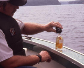
Figure 3. Measuring oxygen using the Winkler technique. The brown color is an indication that oxygen is present. A subsequent titration will quantify this oxygen value.
A more important consideration with chemical tests is that of safety. This chemical technique involves the use of very strong acids and bases. The coordinator must decide whether there is risk in allowing volunteers to use potentially deadly chemicals without supervision, especially if children may be in the volunteer household. Certainly adequate precautions should be taken to educate the volunteers on the potential dangers of the chemicals, such as the wearing of protective aprons, gloves and eye protectors. It is imperative that the volunteers are provided a child-proof box in which to store the chemicals.
The alternative to chemical analysis is convenient and safe, but more expensive. This technique involves using an oxygen probe that is lowered to the desired depth and the oxygen concentration directly read off a meter. An oxygen probe generally uses a reducing electrode covered with a oxygen-permeable membrane. Oxygen passing through the membrane is reduced at the electrode, and the resulting current is measured (Golterman and Clymo 1971).
The dissolved oxygen probe is relatively accurate at high and medium oxygen concentrations, but takes increasingly longer times to equilibrate at very low oxygen concentrations, and may indicate slight amounts of oxygen present when there is actually no oxygen. The membrane on the probe needs care and must be replaced periodically. The oxygen readings should also be calibrated against an atmospheric standard each time it is used and periodic calibration against oxygen concentrations determined chemically should also be done to check for accuracy and linearity.
Another method of indirectly determining oxygen depletion would be to suspend a copper chain into the water. As the oxygen is depleted and a reducing environment is produced, reduced sulfur will be found in the water. This sulfur will combine with the copper to produce copper sulfide, a black precipitate on the chain. It takes several hours for a noticeable color change to take place. Volunteers could permanently suspend a chain in the water and then periodically check the extent of a blackened color on the chain. This technique should be considered as a possible surrogate for more expensive and hazardous methods for estimating the rate of oxygen depletion.
Literature Cited
Gannon, J.E. and A.M. Beeton. 1971. The decline of the large zooplankter, Limnocalanus macrurus sars (Copepoda: Calanoida), in Lake Erie. Proc. 14th Conf. Great Lakes Res. p. 2738.
Gliwicz, Z.M. and A. Kowalczewski. 1981. Epilimnetic and hypolimnetic symptoms of eutrophication in Great Mazurian Lakes, Poland. Freshw. Biol. 11: 425433.
Golterman, H.L. and R.S. Clymo. 1971. Methods for chemical analysis of fresh waters. IBP Handbook No 8. Blackwell Scientific Publications.
Hutchinson, G.E. 1957. A treatise on limnology. Vol. 1. Geography, physics, and chemistry. John Wiley & Sons.
Hutchinson, G.E. and H. Löffler. 1956. The thermal classification of lakes. Proc. Nat Acad Sci., Wash. 42: 8486.
Lewis, W.M., Jr. 1983. A revised classification of lakes based on mixing. Can. J. fish. Aquat. Sci. 40:1779-1787.
Lind, O.T. 1985. Handbook of common methods in limnology. Kendall/Hunt.
Rodhe, W. 1975. The SIL founders and our fundament. Verh. Internat. Verein. Limnol. 19: 1625.
Schmidt, W. 1915. Ber den energiegehalt der seen. Mit beispeilen vom lunzer untersee nach messungen mit einen enifachen Temperaturlot. Int. Rev Hydrobiol. Suppl. 6.
Schmidt, W. 1928. Uber Temperature and Stabilitätsverhältnisse von Seen. Geor. Ann. 10: 145177.
Wetzel, R.G. 2001. Limnology. Academic Press.